Built in plotting function for Kernel density Raster. — plot_forage

This function provides a simple way to produce consistent maps of Kernel density plots. Please be aware that the 'basemap', 'rivers' arguments use the following functions: rosm::osm.image() osmdata::opq() which occasional fail during busy server times.

Usage

plot_forage_density(
  kd_raster,
  basemap = TRUE,
  basemap_type = "cartolight",
  trans_fill = TRUE,
  trans_type = "log10",
  axes_units = TRUE,
  scalebar = TRUE,
  scalebar_loc = "tl",
  north_arrow = TRUE,
  north_arrow_loc = "br",
  north_arrow_size = 0.75,
  wgs = TRUE,
  guide = TRUE,
  catchment = NULL,
  rivers = FALSE,
  plot_extent = NULL,
  attribute = TRUE,
  guide_width = NULL,
  mask_fill = "grey50"
)

Arguments

kd_raster: Kernel Density raster generated from the beavertools::forage_density()
basemap: Boolean, include an OSM basemap. (optional)
basemap_type: Character vector for osm map type. for options see rosm::osm.types()
trans_fill: Boolean to transform the colourmap - visualisation general better when TRUE (the default)
trans_type: Character vector for the type of transform.
axes_units: Boolean to include coordinate values on axis.
scalebar: Boolean to include a scalebar.
scalebar_loc: character vector for the scalebar location one of:'tl', 'bl', 'tr', 'br' Meaning "top left" etc.
north_arrow: Boolean to include a north arrow
north_arrow_loc: character vector for the arrow location one of:'tl', 'bl', 'tr', 'br' Meaning "top left" etc.
north_arrow_size: numeric vector for the arrow
wgs: Boolean to transform coordinate reference system (CRS) to WGS84 (EPSG:4326)
guide: Boolean to include a legend
catchment: An sf object or an sf-readable file. See sf::st_drivers() for available drivers. This feature should be a boundary such as a catchment or Area of interest. It is used to mask the map region outside of desired AOI.
rivers: Boolean to include river lines (downloaded automatcally using the osmdata package) OR a river network of class 'sf' which can be generated beforehand using beavertools::get_rivers().
plot_extent: 'bbox', 'sf' or 'sp' object used to set the plot extent.
attribute: Boolean to include an open street map attribution.
guide_width: numeric vector for the width of the legend.
mask_fill: character vector for the fill colour of the catchment mask.

Value

ggplot object of Kernel Density Map

Examples

# Here we filter the filter the built in 2019-2020 ROBT feeding sign data `RivOtter_FeedSigns`
# Then pipe this 'sf' object to forage_density.

ROBT_201920 <- RivOtter_FeedSigns %>%
dplyr::filter(SurveySeason == "2019 - 2020")%>%
  forage_density(., 'FeedCat')
#> No value supplied for "kd_extent" argument: default extent will be used
#> 
#> calculating weighted kde

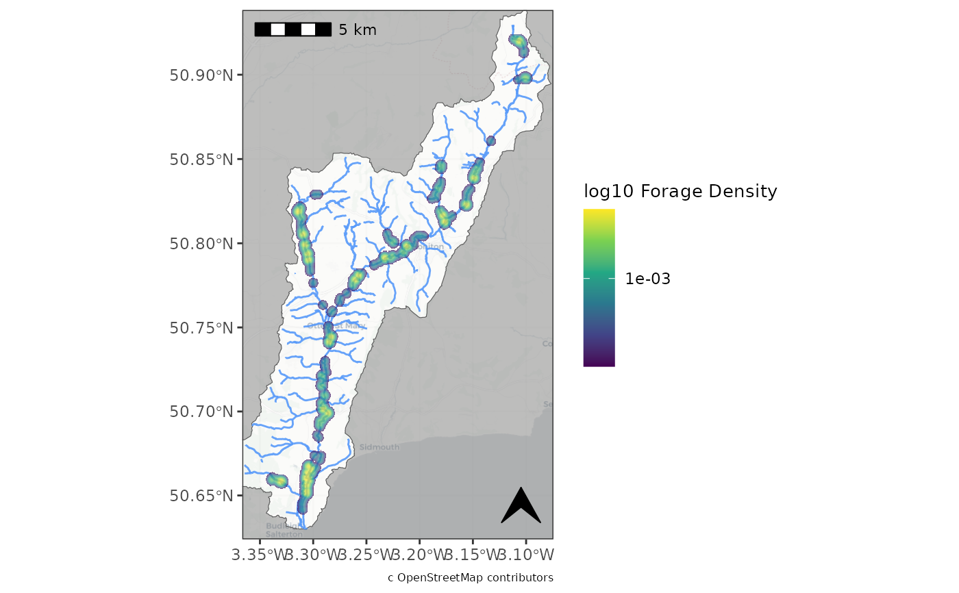
# Now we plot the raster with plot_forage_density
plot_forage_density(ROBT_201920, catchment = RivOtter_Catch_Area, rivers = TRUE,
                                     trans_fill=TRUE)
#> Warning: attribute variables are assumed to be spatially constant throughout all geometries
#> Warning: attribute variables are assumed to be spatially constant throughout all geometries
#> Zoom: 11
#> Fetching 12 missing tiles
#> 
  |                                                                            
  |                                                                      |   0%
  |                                                                            
  |======                                                                |   8%
  |                                                                            
  |============                                                          |  17%
  |                                                                            
  |==================                                                    |  25%
  |                                                                            
  |=======================                                               |  33%
  |                                                                            
  |=============================                                         |  42%
  |                                                                            
  |===================================                                   |  50%
  |                                                                            
  |=========================================                             |  58%
  |                                                                            
  |===============================================                       |  67%
  |                                                                            
  |====================================================                  |  75%
  |                                                                            
  |==========================================================            |  83%
  |                                                                            
  |================================================================      |  92%
  |                                                                            
  |======================================================================| 100%
#> ...complete!
#> Warning: Removed 1390775 rows containing missing values or values outside the scale
#> range (`geom_raster()`).